Oncology Bioinformatics project tutorial-Differential gene expression and Biomarker discovery analysis using Colorectal Cancer dataset

This tutorial involves practical use of Bioinformatics on a Real World dataset as its meant to provide most realistic experience in performing the Differential expression analysis using tens of thousands of gene transcripts from normal and colorectal cancer tissues. The tutorial is based on R and RStudio as software for the implementation. Prerequisites are that you have installed R/Rstudio(you may find more information here — https://posit.co/products/open-source/rstudio/)
Before i start, here is some information about the dataset. First download the dataset design file here : https://www.ebi.ac.uk/gxa/experiments/E-GEOD-50760/Experiment%20Design by clicking the download button on the right.
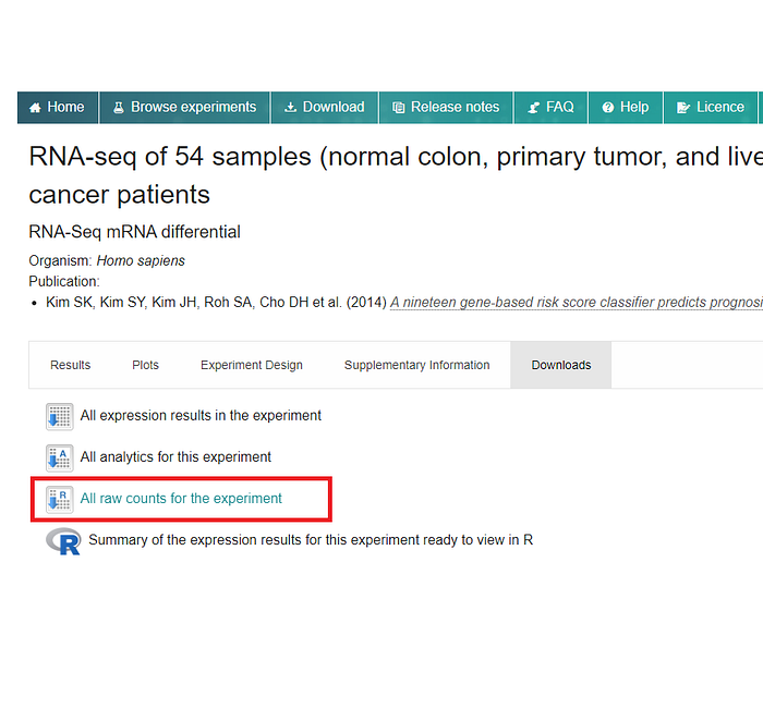
Originating from BioStudy E-GEOD-50760 retrieved from ebi.ac.uk, the actual RNAseq counts dataset may be found here https://www.ebi.ac.uk/gxa/experiments/E-GEOD-50760/Downloads.
This is the dataset interface and the “All raw counts for the experiment” is the file to download for this tutorial

For this tutorial, the Raw counts of gene expressions in (RNA-seq) will be used (i will explain later why).
The dataset is based on an actual study: “Kim SK, Kim SY, Kim JH, Roh SA, Cho DH et al. (2014) A nineteen gene-based risk score classifier predicts prognosis of colorectal cancer patients”.
The dataset contains RNA-seq data from 18 subjects, but sampled (and this is very important) from different tissues of these subjects, normal large intestine tissue, primary colon cancer and progressive liver metastasis (colon originating)[1]. Having that said that, the final number of samples is actually 54[1]. For this tutorial 37 relevant samples, 18 normal and 19 primary colon cancer samples will be used. Why these? Well the basic logic for any potential biomarker discovery is to compare the cancer samples to non-cancer samples and see the differences in their gene expressions.
The cancer samples vs normal samples will be compared across more than 50 000 genes and we want to identify the expression differences between then (the most important ones).
Why is it important that these samples both normal and cancer samples are taken from the same subjects? Because this design limits the confounding variables that could affect the analysis (most other variables in this setting are fixed), enabling better causal inference of potential oncogenes (this will be discussed further).
The DESeq2 package (Bioconductor) will be used to perform the differential expression analysis, identifying a few potentially relevant genes for the disease from a dataset of over 50 000.
Lets install the packages and load the experiment and dataset files and see how they look in R (RStudio)!
#install DESeq2 using Bioconductor
if (!require('BiocManager', quietly = TRUE))
  install.packages('BiocManager')

BiocManager::install('DESeq2')

#Install EnhancedVolcano using Bioconductor
if (!require('BiocManager', quietly = TRUE))
  install.packages('BiocManager')

BiocManager::install('EnhancedVolcano')


library(DESeq2)
library(EnhancedVolcano)
#Load the file containing the experiment design
#'path'=location of the file
design <- read.delim('path/E-GEOD-50760-experiment-design.tsv')


#Load raw counts data
#'path'=location of the file
raw.counts <- read.delim('path/E-GEOD-50760-raw-counts.tsv')
The packages are installed directly from Bioconductor using BiocManager::install() and can not be installed using install.packages().
Keep in mind that ‘path’ word should be replaced with the path of the file location on you computer (eg. ‘C/User/Desktop/E-GEOD-50760-experiment-design.tsv'). The result of the code is packages installed and experiment design file and raw counts loaded. You might wonder why is the experiment design file loaded in addition to the raw counts data. This is very important as the experiment design file contains the Metadata which is needed for Deseq analysis.
Key takeaway: DESeq2 analysis required both the raw counts and the Metadata for the analysis to be run properly.
The data wrangling. Before the data wrangling is started lets discuss the design of the experiment and this analysis.
Simply type
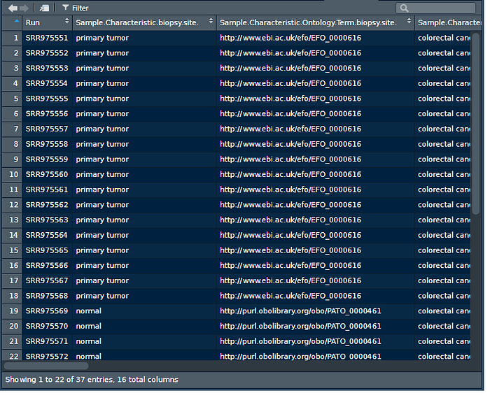
View(design)
As it can be seen the first 18 samples are primary tumors (colorectal cancer) and the next 19 are normal and then the rest are liver metastasis samples. For this tutorial we will use only the first 37, so primary tumor and normal samples. Remember this information, it will be needed for the data wrangling.
Now lets view the raw counts dataset and make sure the counts data is there.
View(raw.counts)
Now that all the data is confirmed, validated and examined, the data wrangling part can be started.
#This file is important because it contatin columns relating samples with phenotypes
design=design[1:37,]


#Create labels for normal and primary cancer samples
label1=rep(c('cancer'),18)
label2=rep(c('normal'),19)
labels=c(label1,label2)


#Load the genetable
#Select the variables of interest data and add gene names
dataset=raw.counts[,c('Gene.Name',design$Run)]
genetable=raw.counts[,design$Run]


#Create the metadata dataframe
Metadata = data.frame(id=design$Run,type=labels)
As it can be seen i manually created the labels using the information from the design object and added the labels to Meta-data object.
The raw.counts object which contains RNA expression raw counts and Gene IDs is used to create new genetable which contains only the 37 samples of interest (this is achieved using design$Run which contains string names for the samples of interest). The genetable the Meta-data objects will provide the raw counts and labels and SRR ids information to the DESeq algorithm during the analysis.
Performing DEseq analysis
#Perform DESeq analysus
dds = DESeqDataSetFromMatrix(genetable,Metadata,~type)
dds <- DESeq(dds)
The DESeq code is fairly simple, its takes only two steps, making the DESeqDataSet and using the DESeq() fuunction on it, however the DESeq is highly complex algorithm it performs many calculations on large datasets (in this case over 50 000 genes.
Having said that, it may take a while for R to finalize all the analyses and you should receive messages in the console that all these analyses are running.
Here are some calculations the DESeq is running…
- Size factor calculation
- Gene-wise dispersion calculation
- Dispersion fit
- Shrinking towards the curve estimation
and other details.
#Create DESeq results object using Benjamini-Hochberg correction
res=results(object = dds, contrast = c('type','cancer','normal'),
            pAdjustMethod = 'BH',alpha = 0.000001)
row.names(res)=dataset$Gene.Name
summary(res)
The output:
>Out:
out of 40166 with nonzero total read count
adjusted p-value < 1e-06
LFC > 0 (up)       : 121, 0.3%
LFC < 0 (down)     : 30, 0.075%
outliers [1]       : 0, 0%
low counts [2]     : 17491, 44%
(mean count < 1)
[1] see 'cooksCutoff' argument of ?results
[2] see 'independentFiltering' argument of ?results
After that the results() function is used to derive and summarize DESeq results. Notice how i set the alpha threshold to p<0.000001. Lets analyze the results…
Out of 40166 non-zero gene counts there are 121 or 0.3% or upregulated genes and 30 or 0.075% of down regulated genes. So that would be around 151 genes of interest out of over 50 000. First conclusions is that there are much more upregulated genes of interest as potential causal factors for this type of cancer, but the 30 downregulated are not something to ignore either.
One thing is very important and that is the multiple testing correction procedure. Over 40 000 nonzero genes means that the analysis will include over 40 000 hypothesis tests. FWER or family wise error rates occurs at high rates in these situations, finding positive results by random is almost certain if multiple correction procedure is implemented. That's why DESeq always has some multiple correction procedures.
I added the pAdjustMethod = ‘BH’, and this means using Benjamini-Hochberg correction, i did this on purpose so you can see how to implement the multiple testing procedures, even tough its implemented by default. But multiple testing procedure is very important in this case and i want a more robust method implemented. Therefore i will use the Holm multiple testing adjustment, which is going to be more robust on FWER.
#Create DESeq results object using Holmr correction
res=results(object = dds, contrast = c('type','cancer','normal'),
            pAdjustMethod = 'holm', alpha = 0.000001)
row.names(res)=dataset$Gene.Name
summary(res)
The output:
out of 40166 with nonzero total read count
adjusted p-value < 1e-06
LFC > 0 (up)       : 46, 0.11%
LFC < 0 (down)     : 11, 0.027%
outliers [1]       : 0, 0%
low counts [2]     : 18251, 45%
(mean count < 1)
[1] see 'cooksCutoff' argument of ?results
[2] see 'independentFiltering' argument of ?results
Ok as we can see the Holm multiple testing adjustment is much more robust and has eliminated almost 100 genes previously marked as significant. Now only 57 remain with significant differences between cancer and normal samples (46 upregulated or 0.11%, 11 down-regulated or 0.027%). Now you can see one of the experiences of RNA Differential expression analysis is finding as little as 0.027% of interesting down-regulated genes which would be a bit more then 1 in 3000 genes.
Key takeaway : When studying large number of genes such as tens of thousands, the tests should be very conservative in terms of multiple testing adjustments.
First test volcano plot
#Create publication grade volcano plot with marked genes of interest
EnhancedVolcano(res,
                lab = dataset$Gene.Name,
                x = 'log2FoldChange',
                y = 'pvalue',
                pCutoff = 10e-5,
                FCcutoff = 1.333,
                xlim = c(-5.7, 5.7),
                ylim = c(0, -log10(10.2e-12)),
                pointSize = 1.3,
                labSize = 2.6,
                title = 'The results',
                subtitle = 'Differential expression analysis',
                caption = 'log2fc cutoff=1.333; p value cutof=10e-5',
                legendPosition = "right",
                legendLabSize = 14,
                col = c('lightblue', 'orange', 'blue', 'red2'),
                colAlpha = 0.6,
                drawConnectors = TRUE,
                hline = c(10e-8),
                widthConnectors = 0.5)
Intepretation principle of the volcano plots is quite intuitive. The plot is segmented into areas which have significant and non-significant observations based on p values and log2fold changes.
Better volcano plot
#Create publication grade volcanoplot with marked genes of interest
EnhancedVolcano(res,
                lab = dataset$Gene.Name,
                x = 'log2FoldChange',
                y = 'padj',
                pCutoff = 10e-7,
                FCcutoff = 2.5,
                xlim = c(-5.7, 5.7),
                ylim = c(0, -log10(10.2e-12)),
                pointSize = 1.3,
                labSize = 2.6,
                title = 'The results',
                subtitle = 'Differential expression analysis',
                caption = 'log2fc cutoff=1.333; p value cutof=10e-6',
                legendPosition = "right",
                legendLabSize = 14,
                col = c('lightblue', 'orange', 'blue', 'red2'),
                colAlpha = 0.6,
                drawConnectors = TRUE,
                hline = c(10e-8),
                widthConnectors = 0.5)
Key takeaway: Generally better to use padj for y axis when dealing with large number of transcripts.
Tidy up and output the results as a table
#Create the final dataframe consisting of ordered deseq results based on log2fc
resord=as.data.frame(res)
finaltable1=resord[order(resord$padj),]
write.table(finaltable1, file = 'finaltable.csv', sep = ',',
            col.names = NA)
The last part of the tutorial is to practice interpretaion.
The most interesting genes are at the top. Final interpretation would be that the interesting genes were identified starting with COL11A1, CEMIP, ADAM12, MMP1, OTOP3 and further experimental research would be needed to conclude if any of these are potential cancer treatment targets.
Final takeaway:DESeq is very practical and efficent in taking large complex datasets and identifying potential Biomarkers for disease of interest. Differentail expression analysis is specific for having large amounts of tests and the p adjusted values playa key role in finding the differentialy expressed transcripts.
Note: The tutorial and the practice interpretations are meant for learning purposes.
By
Darko Medin, Data Science, Biostatistics and Bioinformatis expert
References:
The data sources : Kim SK, Kim SY, Kim JH, Roh SA, Cho DH et al. (2014) A nineteen gene-based risk score classifier predicts prognosis of colorectal cancer patients.
Software:
Tutorial Github repo : https://github.com/DarkoMedin/Oncology---RNAseq-Differential-Expression-Bioinformatics
Multiple correction procedures:
- Benjamini Y. Hochberg Y. Controlling the false discovery rate: a practical and powerful approach to multiple testing. Journal of the Royal Statistical Society. (1995)
- Holm S. A simple sequentially rejective multiple test procedure. Scandinavian Journal of Statistics. (1979)
